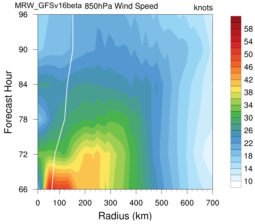
12.3. Plotting Radial WS with Leading Times

This script plots the 850 hPa radial wind speed with leading times. The radialAvg.ncl needs to be staged to the same directory as the example ncl script below.

; Purpose: plot the 850 hPa radial wind speed variation with leading times from UFS Medium-Range Weather App model run outputs, as well as the GFDL tc-tracker outputs. The radialAvg.ncl needs to be staged to the same directory from UFS Medium-Range Weather App model run outputs, as well as the GFDL tc-tracker outputs.
; Usage: ncl tc_radial_time_RMW.ncl
; Author: Xia Sun, xia.sun@noaa.gov, Oct 15, 2020

loadscript( "radialAvg.ncl")

begin

; Define plot name
pngname="ufs_GFSv16beta_radial_ws_time_plot"
wks=gsn_open_wks("png", pngname)

; Read GFSv16beta vortex tracker results
tcfile="GFSv16beta/fort.69"
delim=","
tclines=asciiread(tcfile, -1, "string")
leadtimestr=tointeger(str_get_field(tclines, 6, delim))
tclatstr=str_get_field(tclines, 7, delim)
tclonstr=str_get_field(tclines, 8, delim)
tcRMWstr=str_get_field(tclines, 20, delim)
tcRMW=tofloat(tcRMWstr)


tcdimsize=dimsizes(leadtimestr)-1
critstr=str_get_field(tclines, 12, delim)
crit=toint(critstr)
count=0
newtcRMW=new((/29/),float)
do i=0,tcdimsize,1

    if(crit(i).eq.34) then
        newtcRMW(count)=tcRMW(i)
        count=count+1
    end if
end do

do i=0,tcdimsize,1
    if(leadtimestr(i).eq.leadtime) then
        tclat=tofloat(str_get_cols(tclatstr(i), 0, 3))*0.1
        tclon=tofloat(str_get_cols(tclonstr(i), 0, 4))*0.1
        print(tclat)
        print(tclon)
    end if
end do
psminlat= tclat
psminlon= tclon*(-1)+360

; Use wgrib2 to convert all the GFSPRS* outputs to NetCDF (nc) format, and read in all the nc files
ncfili=systemfunc("ls GFSv16beta/GFSPRS.GrbF*.nc")
ncfiles=addfiles(ncfili,"r")

UGRD850=ncfiles[:]->UGRD_850mb
VGRD850=ncfiles[:]->VGRD_850mb
WS850=(wind_speed(UGRD850,VGRD850))*1.944


; Make an array for leading time after landfall from f66 to f120
time=(/66,72,78,84,90,96,102,108,114,120/)
dsizes=dimsizes(UGRD850)

; Define a new array for 850 hPa wind speed, /Pressure, latitude, longitude/
verTMP=new((/dsizes(0),dsizes(1),dsizes(2)/),float)
verTMP!0 ="Pressure"
verTMP&Pressure=time ;Trick to replace pressure with leading time data
verTMP&Pressure@units="hPa"
verTMP!1="latitude"
verTMP&latitude=UGRD850&latitude
verTMP!2="longitude"
verTMP&longitude=UGRD850&longitude

verTMP(0,:,:)=(/WS850(0,:,:)/)
verTMP(1,:,:)=(/WS850(1,:,:)/)
verTMP(2,:,:)=(/WS850(2,:,:)/)
verTMP(3,:,:)=(/WS850(3,:,:)/)
verTMP(4,:,:)=(/WS850(4,:,:)/)
verTMP(5,:,:)=(/WS850(5,:,:)/)
verTMP(6,:,:)=(/WS850(6,:,:)/)
verTMP(7,:,:)=(/WS850(7,:,:)/)
verTMP(8,:,:)=(/WS850(8,:,:)/)
verTMP(9,:,:)=(/WS850(9,:,:)/)

; Using the radialAvg3D function from the radialAvg.ncl
outerRad=700.
mergeInnerBins=True
radiaverWS850=radialAvg3D(verTMP(:,:,:),lat,lon,verTMP&Pressure,psminlat,psminlon,outerRad,mergeInnerBins)
radiaverWS850f=tofloat(radiaverWS850)
copy_VarCoords(radiaverWS850, radiaverWS850f)



; Plot the contour field of wind speed at 850hPa
resx=True
resx@gsnDraw = False
resx@gsnFrame=False
 resx@cnFillOn             = True            ; turn on color fill
resx@cnLinesOn            = False        ; turn lines on/off         ; True is default
resx@cnLineLabelsOn       = False          ; turn line labels on/off   ; True is default
resx@cnFillPalette="WhiteBlueGreenYellowRed";"temp_19lev"
resx@cnLevelSelectionMode="ManualLevels"
 resx@tmXTOn=False
 resx@tmYROn=False
 resx@lbOrientation="Vertical"
resx@tiYAxisString ="Forecast Hour"
resx@tiXAxisString="Radius (km)"
radiaverWS850f@units="knots"
radiaverWS850f@long_name="MRW_GFSv16beta 850hPa Wind Speed"
resx@cnLevelSelectionMode="ManualLevels"
resx@cnMinLevelValF= 10
resx@cnMaxLevelValF= 60
resx@cnLevelSpacingF= 2
resx@trYMinF=66
resx@trYMaxF=96
resx@tmYLMode="Explicit"
resx@tmYLValues=(/66,72,78,84,90,96/)
resx@tmYLLabels=(/66,72,78,84,90,96/)
plot=gsn_csm_contour(wks, radiaverWS850f(0:5,:), resx)


; Overlay the white line of radius of the maximum wind (RMW) to the wind speed contour plot
res=True
res@gsnDraw = False
res@gsnFrame=False
res@xyLineColors        = (/"white"/)
res@xyLineThicknesses   = (/5.0/)
plotxy=gsn_csm_xy(wks, newtcRMW(10:15), time(0:5),res)
overlay(plot, plotxy)
draw(plot)
frame(wks)

end